Essential Principles of Microeconomics and Macroeconomics

Macroeconomics vs. Microeconomics

Macroeconomics examines the behavior of the whole economy, while Microeconomics focuses on individual consumers and firms.

Fundamental Economic Questions: WHAT-HOW-WHO?

Adam Smith introduced the concept of the “invisible hand” in markets. Market failures can arise from government intervention, among other reasons.

Profit = Revenue – Cost

Efficiency vs. Equity

• Efficiency is concerned with the optimal production and allocation of resources, given existing factors of production.
• Equity refers to how equally resources are distributed throughout society.

Key Economic Principles:

• There are gains from trade.
• Markets tend to move toward equilibrium.
• Markets usually lead to efficiency.
• Resources should be used efficiently.

Scarcity and Opportunity Cost

• Scarcity: There are not enough goods or services to satisfy everyone’s wants.
• Opportunity Cost: The value of the best alternative forgone when making a choice.

Marginal Analysis: Making decisions at the margin involves considering whether to do a bit more or less of something.

Market Failure: Occurs when individual actions have side effects that are not properly taken into account by the market.

Supply and Demand

• Law of Demand: At a lower price, more people want the product.
• Law of Supply: The higher the quantity supplied, the higher the price (coordinated).
• Movement Along the Curve (Change in Quantity Demanded/Supplied): Related to price changes.
• Shift in Demand: Caused by external factors (not price), such as changes in the prices of related goods, tastes, or income.
• Demand: The market’s desire to purchase a good.
• Quantity Demanded/Supplied (QD/QS): The amount people will buy or sell.
• Normal Good: Demand increases with higher income (e.g., air travel, restaurants).
• Inferior Good: Demand decreases with higher income (e.g., supermarket goods, used cars).

Surplus and Shortage

• Surplus: Excess supply; supply is high, and demand is low.
• Shortage: Excess demand; Quantity Demanded (QD) is higher than Quantity Supplied (QS).

Consumer and Producer Surplus

• Consumer Surplus: The difference between a consumer’s willingness to pay and the actual price. Consumer Surplus (CS) is high when the price is low.
• Producer Surplus: The difference between the price a producer is willing to accept and the price received.
• Total Surplus: Consumer Surplus + Producer Surplus. Total surplus is maximized when the market is in equilibrium.

Price Controls

Price Control: A legal restriction imposed by the government to regulate prices. Price controls make markets less efficient.

• Binding Price Ceiling: Designed to keep prices low.
• Price Ceiling: The maximum price sellers can charge (equilibrium is above the ceiling).
• Price Floor: The minimum price buyers are required to pay.

Elasticity

Price Elasticity of Demand (PED): Measures the responsiveness of demand to a change in price.

% Change in Quantity Demanded / % Change in Price

• Elastic: PED > 1
• Inelastic: PED < 1
• Unit Elastic: PED = 1

Factors Affecting PED: Availability of substitutes, necessity vs. luxury, time.

• Perfectly Inelastic Demand: Quantity demanded does not respond to price changes (vertical demand curve).
• Perfectly Elastic Demand: Any price increase causes quantity demanded to drop to zero (horizontal demand curve).

Price Effect: Each unit sells at a higher price.

Quantity Effect: Fewer units are sold.

Cross-Price Elasticity of Demand (XED): Measures the responsiveness of one product’s demand to changes in the price of another product.

% Change in Quantity Demanded of Good A / % Change in Price of Good B

• Substitutes: XED > 0
• Complements: XED < 0

Income Elasticity of Demand (YED): Measures the responsiveness of demand to changes in income.

% Change in Quantity Demanded / % Change in Income

• Normal Good: YED > 0
• Inferior Good: YED < 0

Price Elasticity of Supply (PES): Measures the responsiveness of supply to changes in price.

% Change in Quantity Supplied / % Change in Price

Midpoint Method:

When price decreases, quantity increases.

Production and Costs

Total Product Curve: Shows the quantity produced in relation to the quantity of an input.

Marginal Product of Labor: The slope of the total product of labor curve. Change in Quantity Produced / Change in Quantity of Labor

Diminishing Returns: When an increase in the quantity of an input leads to a decline in its marginal product.

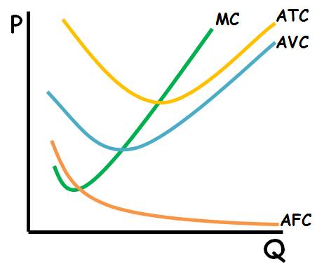
• Fixed Cost: Cost that does not depend on the quantity produced.
• Variable Cost: Cost that depends on the quantity produced.
• Total Cost: Fixed Cost + Variable Cost

In the short run, fixed costs are unchangeable; in the long run, they become variable costs.

Marginal Cost: Usually increases due to diminishing returns. Change in Total Cost / Change in Quantity Produced

Constant Marginal Cost: When the cost of producing an additional unit is the same as the previous unit.

Decreasing Marginal Cost: Can occur due to learning effects (workers gain experience and make fewer mistakes).

• Average Fixed Cost: Fixed Cost / Quantity Produced
• Average Variable Cost: Variable Cost / Quantity Produced
• Average Total Cost: Total Cost / Quantity Produced = Average Fixed Cost + Average Variable Cost

Spreading Effect: The larger the output, the greater the quantity over which fixed cost is spread, leading to lower average fixed cost.

Diminishing Returns Effect: The larger the output, the greater the variable cost required to produce additional units, leading to higher average variable cost.

Economies of Scale: Exist when long-run average total cost decreases as output increases.

Diseconomies of Scale: Occur when long-run average total cost increases as output increases. Constant returns to scale occur when costs do not change with output.

• Short Run: Some inputs are fixed costs and variable costs. The average total cost curve slopes upward due to diminishing returns.
• Long Run: All inputs are variable.

If Marginal Cost is greater than Average Total Cost, then Average Variable Cost is increasing. If Marginal Cost is equal to Average Variable Cost, then Average Variable Cost is at its minimum.

Opportunity Cost and Profit

Opportunity Cost: The value of the next-best alternative; the value of forgone benefits.

• Explicit Costs: Out-of-pocket costs; actual spending of money.
• Implicit Costs: Opportunity costs that do not require spending money.

• Accounting Profit: Revenue – Explicit Cost
• Economic Profit: Revenue – (Explicit Cost + Implicit Cost)

Capital: The value of a business’s assets (equipment, buildings, tools, inventory, financial assets).

Implicit Cost of Capital: The opportunity cost of the capital used by a business.

Sunk Cost: A cost that has already been incurred and is unchangeable. Sunk costs have no effect on future costs and benefits.

Marginal Cost: The additional cost incurred by producing one more unit.

Marginal Revenue: The additional revenue earned from producing one more unit. The marginal revenue curve shows how the revenue from producing one more unit depends on the quantity already produced.

Optimal Quantity: The quantity that generates the maximum possible total profit.

Golden Rule: Optimal Quantity = Quantity at which Marginal Revenue (MR) = Marginal Cost (MC)

Quiz Notes:

• Economic profit is less than accounting profit if implicit costs exist.
• Profit is the difference between total revenue and total cost.
• Accounting profit is not the only measure of cost.
• Marginal benefit is the amount by which an additional unit of activity increases total benefits.
• According to the optimal output rule, if marginal benefit is less than marginal cost, an activity should be reduced.

Market Structures

Price-Taking Producer: A producer whose actions have no effect on the market price of the good sold (e.g., Samsung, a brand that follows the price of the top brand, benefits from high economies of scale, produces less, and charges higher prices).

Perfectly Competitive Market: Everyone is a price-taker. MC = MR.

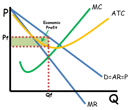
In perfect competition, if Average Total Cost (ATC) is above P = MR, there is a loss (no profit).

Monopoly: Only one firm in the market, with no substitutes or competitors (e.g., Google). Monopolies raise prices and decrease production. Governments often try to break up monopolies due to economic inefficiency (e.g., by imposing price ceilings).

Natural Monopoly: Average cost is always decreasing (e.g., electricity).

Price Discrimination: Offering discounts or different prices depending on the type of consumer (e.g., students, children, professionals, pregnant women).

Perfect Price Discrimination: Charging different prices based on each consumer’s willingness to pay.

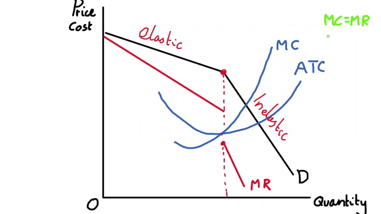
In a monopoly, Marginal Revenue is always below the price. Monopolies decrease prices to sell more units, causing the marginal revenue curve to be below the demand curve.

Market Power: The ability of a monopolist to raise the price of a product above the competitive level.

Oligopoly

Oligopoly: A market with a few firms, where there is strategic interdependence. Firms must consider rivals’ reactions before making decisions. Economies of scale make it not worthwhile to increase prices. Prices tend to stay constant over time.

Kinked Demand Curve: It is not worthwhile to increase prices. There are a small number of producers. Products can be identical or differentiated. Entry to the market is difficult.

How to determine if a market is an oligopoly:

HHI (Herfindahl-Hirschman Index): The sum of the squares of each firm’s market share. For example: (60%)^2 + (30%)^2 = … A single firm (monopoly) has an HHI of 100^2 = 10,000.

• HHI < 1,000: Strongly competitive market
• 1,000 < HHI < 1,800: Somewhat competitive market
• HHI > 1,800: Oligopoly

Collusion: Two firms agree to fix prices to raise profits.

Cartel: The strongest form of collusion. Cartels are illegal, unstable, and involve overt collusion (e.g., OPEC).

Noncooperative Behavior: Quantity competition or price competition. Marginal cost is relevant in perfect competition.

Interdependence: One firm’s decisions impact the profits of other firms.

Game Theory: A tool to analyze situations with interdependent decisions.

Payoff: Profit; the outcome of the game.

Coordination Game; Prisoner’s Dilemma: Both players have an incentive to cheat. The Nash equilibrium is a non-cooperative solution. The dominant strategy for both players is to confess (the best action regardless of the other player’s action).

Tacit Collusion: An unwritten or unspoken agreement to collude.

Antitrust Laws: Government regulations to prevent oligopolists from colluding or behaving like monopolists.

Price Leadership: Smaller firms silently agree to charge the same price as the largest firm.

Non-Price Competition: Using advertising or other means to increase sales.

Battle of the Sexes: A coordination game.

Tit for Tat: After cooperating in the first round, a player copies the other player’s strategy.

Backward Induction: A method to predict outcomes of dynamic games. There can be two Nash equilibria.