Statistical Methods for Data Reduction and Classification

Posted on Mar 13, 2025 in Mathematics

Linear Regression

Linear Regression: Finds the best line that summarizes the relationship between two variables. (Imagine a bunch of dots and a line representing the relationship).

Dimensionality Reduction

A large number of variables results in a dispersion matrix that is too large to study. Dimensionality reduction reduces the number of variables to a few. Why?

• Simpler Analysis: Fewer features make it easier to find patterns.
• Faster Processing (e.g., Trading).
• Better Visualization: It’s easier to visualize 2 features than 100.

Correlation Analysis

Correlation analysis tells the strength and direction of the relationship between two variables (-1 to 1). If x increases and y increases, then r is positive. If r is closer to 1, x and y are positively correlated. If r is closer to -1, x and y are negatively correlated. If r is closer to 0, there is a weak relationship between x and y.

How Can Correlation Help Reduce Dimensionality?

Imagine you have many features (X1, X2, …, Xn), and you want to reduce them to a smaller set while keeping the important ones. Here are the steps to reduce features using correlation:

1. Find Correlation Between Features: Compare each feature pair (e.g., X1 & X2, X1 & X3) to check if they are highly correlated.
2. Compare Correlation With Target Variable (Y): If two features are correlated, check which one has a stronger relationship with Y. Keep the one with a stronger correlation and remove the weaker one.

Probable Error (PE_r)

1. A limitation of correlation is that it doesn’t consider data size.
   1. A correlation of 0.5 in 20 samples is weaker than 0.5 in 10,000 samples.
   2. Probable Error (PE_r) helps adjust correlation strength based on sample size.
2. Formula: PE_r = 0.674 × (1 – r²) / √n
3. where r = correlation coefficient and n = number of data points. If:
   1. r > 6 × PE_r → Strong correlation
   2. r < 6 x PE_r
4. Example: If you have a large dataset, even a small correlation (e.g., 0.1) could be meaningful!
5. Analyze the “correlation.” Why is a correlation of 0.5 with 20 samples *less* significant than a correlation of 0.5 with 10000 samples?

Principal Component Analysis (PCA) – Important

1. PCA is a technique used to reduce the number of variables (dimensions) in a dataset while keeping the most important information.
2. Why Do We Need PCA?
   1. Too many variables (features) can make analysis complex and slow.
   2. Some features are redundant (they contain similar information).
   3. PCA helps find a smaller set of “important” variables that still explain most of the data.
3. How PCA Works
   1. Collect Data: Imagine you have a dataset with multiple variables (e.g., height, weight, age, income).
   2. Create a Covariance Matrix: This matrix shows how variables are related to each other.
   3. Find Eigenvalues & Eigenvectors:
      1. Eigenvalues tell us how much information (variance) each new feature (Principal Component) captures.
      2. Eigenvectors represent the directions of the new features.
   4. Choose Principal Components:
      1. We keep only the most important components (those with the largest eigenvalues).
      2. These new features are combinations of original variables but capture most of the important patterns in the data.
4. How PCA Works – Covariance Matrix
   1. A covariance matrix is a table that shows how different variables in your dataset are related to each other. Example:
      1. Imagine you have a dataset with Height and Weight of people.
         1. If taller people tend to be heavier, then Height and Weight have a positive covariance (they increase together).
         2. If one variable goes up while the other goes down, the covariance is negative.
         3. If they are completely unrelated, covariance is close to zero.
   2. A covariance matrix stores these relationships for all variables in a dataset.
   3. Covariance Matrix = [ Cov(Height, Height) Cov(Height, Weight) Cov(Weight, Height) Cov(Weight, Weight)]
5. This helps PCA understand which variables contain similar information so that it can merge them into fewer variables.
6. How PCA Works: YES ON THE TEST. PLEASE FILL THIS SECTION OUT
   1. Eigenvector with covariance matrix
      1. (Know the difference between the two)
   2. Eigenvalues with covariance matrix
      1. Within a three-dimensional graph for both (3-2-2)
   3. Principal Components
   4. Worried how to study this beyond barebones definitions
   5. Pick dimension for new dataset
7. How PCA works – YES ON THE TEST
8. Mutual Information – NOT ON THE TEST (don’t worry about this one)

Week 3

Naive Bayes Classifier

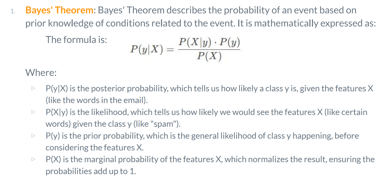
1. The Naive Bayes classifier is a probabilistic machine learning model used for classification tasks.
2. It is based on Bayes’ Theorem and assumes that the features (predictors) are conditionally independent given the class label.
3. This “naive” assumption simplifies the computation, making the algorithm fast and efficient, even for large datasets.

Multinomial Naive Bayes

1. Used for discrete data, such as word counts in text classification.
2. Assumes features represent the frequency of events (e.g., word occurrences).
3. Example: Spam detection, document classification.

Go through the example of Naive Bayes classifier and connect it to the definition. UNDERSTAND IT (YES)

Example of Multinomial Naive Bayes Classifier

1. Imagine you want to classify emails you receive as spam or not spam.
   1. We take all the words in a normal (not scam) email and create a plot (e.g., a histogram) to see how many times each word occurs in the normal email.
   2. We can use the histogram (word count) to calculate the probabilities of seeing each word, given that it was a normal email.
      1. For example, the probability of a word “free” in a normal message = P(free|normal) = the total number of times “free” occurred in normal email (say 5) / the total number of words in a normal email (say 100).
         1. P(free|normal) = 5/100 = 0.05
      2. Similarly, the probability of a word “offer” in a normal message = P(offer|normal) = the total number of times “offer” occurred in normal email (say 8) / the total number of words in a normal email (say 100).
         1. P(offer|normal) = 8/100 = 0.08
   3. Now we make a histogram of all the words that occur in a spam email (to count occurrences of each word).
   4. We can use the histogram (word count) to calculate the probabilities of seeing each word, given that it was a spam email.
      1. For example, the probability of a word “free” in a spam message = P(free|spam) = the total number of times “free” occurred in spam email (say 20) / the total number of words in a spam email (say 50).
         1. P(free|spam) = 20/50 = 0.4
      2. Similarly, the probability of a word “offer” in a spam message = P(offer|spam) = the total number of times “offer” occurred in spam email (say 40) / the total number of words in a spam email (say 50).
         1. P(offer|spam) = 40/50 = 0.8
   5. Now, imagine you got a new email that said “offer!”, and we want to decide if this is a normal email or spam.
   6. We start with an initial guess about the probability that any email, regardless of what it says, is a normal email.
      1. We would estimate this guess from the training data.
      2. For example, since 100 of the 150 emails are normal, P(N) = 100/(100+50) = 0.66
   7. This initial guess that we observe a normal email is called “prior probability.”
   8. Now we multiply that initial guess by the probability that the word “offer” occurs in a normal email.
      1. P(N) × P(offer|normal) = 0.66 × 0.08 = 0.0528
      2. We can think of 0.0528 as the score that “offer” gets if it belongs to the normal email class.
   9. Just like before, we start with an initial guess about the probability that any email, regardless of what it says, is spam.
      1. We would estimate this guess from the training data.
      2. For example, since 50 of the 150 emails are spam, P(S) = 50/(100+50) = 0.33
   10. Now we multiply that initial guess by the probability that the word “offer” occurs in a spam email.
       1. P(S) × P(offer|spam) = 0.33 × 0.8 = 0.264
       2. We can think of 0.264 as the score that “offer” gets if it belongs to the spam class.
   11. Because the score we got for “offer” if it belongs to spam is greater than the score if it belongs to the normal email, we will decide that “offer!” is a spam email. (0.264 > 0.0528)
2. Understand why it goes either to the spam folder or regular folder.

Naive Bayes “Naive” – YES

1. Treats all word orders the same.
   1. For example, the normal email score for “free offer” is the exact same for “offer free.”
      1. P(N) × P(free|normal) × P(offer|normal) = P(N) × P(offer|normal) × P(free|normal)
   2. Treating all word orders the same is different from the real-world use of language.
   3. Naive Bayes ignores all types of grammar and language rules.
   4. By ignoring the relationship between words, Naive Bayes has high bias, but because it works well in practice, it has low variance.

Week 4

K-Means Clustering – YES

1. A partitioning method that divides data into k distinct clusters based on distance to the centroid of a cluster.
   1. Requires the number of clusters (k) to be specified in advance.
   2. Iteratively assigns data points to clusters and updates cluster centroids.

K-Means Clustering Process – YES

1. Initialization: Choose k initial centroids (randomly or using heuristics).
2. Assignment Step: Assign each data point to the nearest centroid.
3. Update Step: Calculate the new centroids as the mean of all data points assigned to each cluster.
4. Repeat: Continue the assignment and update steps until convergence (no change in centroids).
5. Imagine a graph with three clusters of points (bottom left, bottom middle, top right, each has a centroid in the center of the clusters of points).

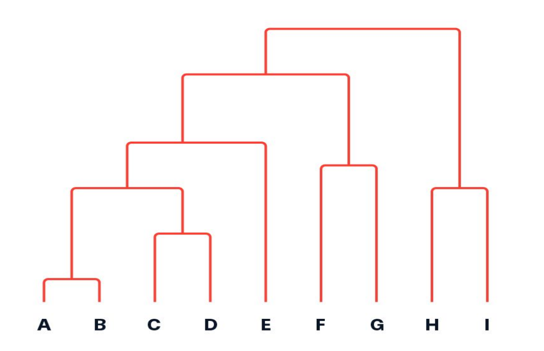
Hierarchical Clustering

1. A method of grouping data points into clusters in a step-by-step manner.
2. It is like creating a family tree of clusters, where similar data points get grouped together as you move up or down the tree.

Key difference between K-means and hierarchical clustering

Agglomerative (Bottom-Up Approach) Hierarchical Clustering

1. Starts with each data point as its own cluster.
2. Merges the two most similar clusters at each step.
3. Stops when all points form a single large cluster.
4. Steps:
   1. Start: Each data point is treated as an individual cluster.
   2. Find the Closest Clusters: Measure the similarity (distance) between all clusters.
   3. Merge: Combine the two closest clusters into one.
   4. Repeat: Keep merging until only one cluster remains or until a set number of clusters is reached.

How do you study the clusters in terms of graphs?

Understand the A B C D E graph in the screenshot that’s also in the slides

Methods, Distance Calculation – NOPE

DBSCAN Explanation

1. DBSCAN (Density-Based Spatial Clustering of Applications with Noise) is a clustering algorithm that groups together points that are close to each other in dense regions while identifying outliers (noise).
   1. No need to specify the number of clusters (unlike K-Means).
   2. Can find clusters of different shapes (not just circular clusters like K-Means).
   3. Detects outliers (points that don’t fit into any cluster).
   4. Core Points: Have at least min_samples points within eps distance.
   5. Boundary Points: Not core points but close to at least one core point.
   6. Noise Points: Not close enough to any cluster (assigned label -1).

DBSCAN example – YES – understand core points to see if you can cluster points together

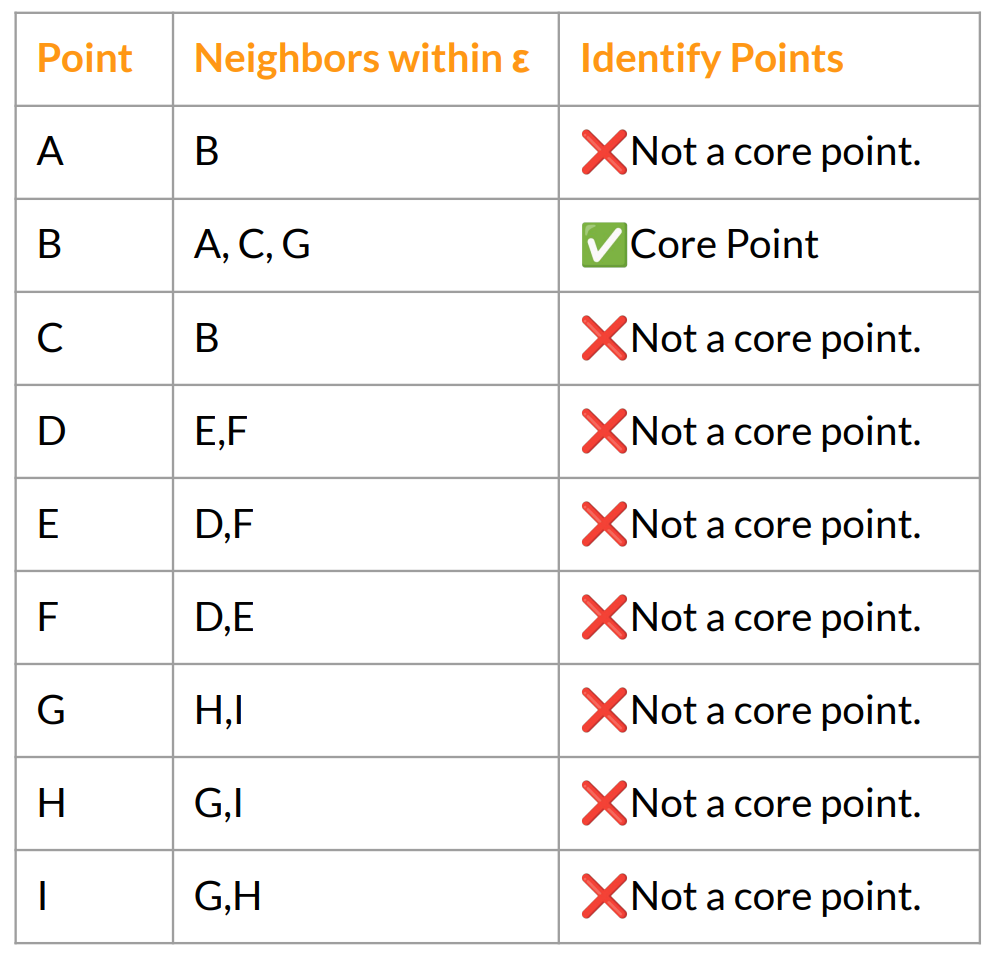
1. Given Dataset: We have the following points: A, B, C, D, E, F, G, H, I. Let’s assume the following neighborhood relationships exist within distance eps (ε):
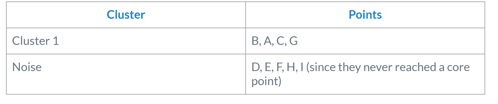
2. Step 2: Start a Cluster from Core Points B is a core point, so it forms a new cluster (Cluster 1). B’s directly reachable points (A, C, G) are added to the cluster. Current Cluster 1: {B, A, C, G}
3. Step 3: Expand the Cluster
   1. We check if any of the new members (A, C, G) are also core points.
   2. C and A are not core points (not enough neighbors), so we don’t expand from them.
   3. G has only 2 neighbors (H, I), which is less than 3, so it is NOT a core point either.
   4. Since there are no more core points, the expansion stops here.
4. Step 4: Identify Remaining Points
   1. D, E, and F are not connected to B’s cluster and form another group where all are neighbors of each other.
   2. None of them are core points (each has only 2 neighbors), so they don’t expand.
   3. They remain unclustered or noise, depending on the dataset structure.